Kinked Demand Curve Model
Here we understand the Kinked Demand Curve Model in detailed.
Do you have similar website/ Product?
Show in this page just for only
$2 (for a month)
0/60
0/180
KINKED DEMAND CURVE MODEL
This model was simultaneously advanced by Paul M. Sweezy in America and R.L. Hall and C.J. Hitch in England to explain the price rigidity in oligopolistic industries.
According to this theory, an oligopolist firm faces a kinked demand curve on the assumption that if it raises its price, its rivals will not raise their prices but if it lowers its price they will definitely lower their prices.
This results in a kink in the demand curve at the prevailing price. At price higher than the prevailing one, demand curve will be more elastic and at prices lower than the prevailing one, demand curve will be less elastic.
Figure-1: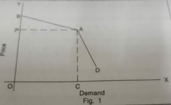
As shown in Figure-1, demand curve faced by an oligopolistic firm is BAD. It has a kink at A. OP or CA is the prevailing price. OC is the output produced and sold at this price. BA segment of this demand curve reflects high degree of elasticity. This implies that if the firm raises its price even slightly, its sales will decline substantially because its rivals do not reduce their prices. However AD segment of the demand curve reflects low degree of elasticity. This implies that if the firm reduces its price even substantially, its sales will increase only slightly, because its rivals also reduce their prices.
Every firm in aims at maximisation of profits. It attains equilibriums at that level of output where marginal cost is equal to marginal revenue. The equilibrium of the firm is defined by the point of the kink. At any point to the left of the kink MC is below MR, while to the right of the kink, MC is greater than MR. Here total profit is maximum at the point of the kink as shown in figure-2.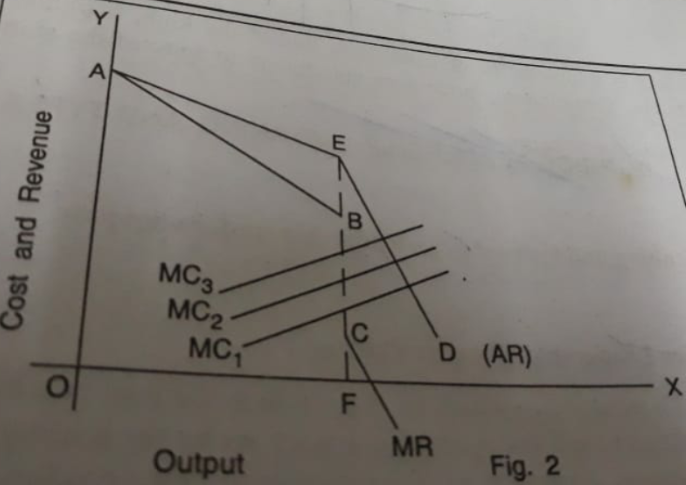
As shown in figure-2, the demand curve (D) has a kink at E. At the kink prevailing price is EF at which OF output is produced. Due to the kink in the demand curve, MR curve is discontinuous, that is MR curve has two segments; segment AB corresponding to upper part of the demand curve (AE) and segment below point C corresponding to the lower part of the demand curve. Thus MR curve is discontinuous between B and C.
As shown in figure-2, Here MC curve (whether MC1 or MC2 or MC3) cuts the MR curve in its discontinuous portion (BC), the price remains stable at EF level, and the equilibrium level of output remains OF. This is known as 'price rigidity'. Price does not change inspite of the shifts in the MC curve.
CONTINUE READING
Kinked Demand Curve Model.
Kinnari
Tech writer at NewsandStory