Nature of Long Run Average Cost Curves (LAC)
Here, we understand with diagram the nature of long run average cost curve in detailed.
Do you have similar website/ Product?
Show in this page just for only
$2 (for a month)
0/60
0/180
Nature of Long Run Average Cost Curves (LAC)
We noted that in long run all costs are variable. Even fixed factors becomes variable. A firm may have many plants, i.e. factories. It can change plant size or its scale of operations in long period of time. The long run problem confronting a business firm is to select the optimum size that is least cost - plant to produced predetermined output. The long run average cost curve (LAC) shows the minimum cost for that level of output. It is derived by joining the tangency points of short run average cost curves. Every SAC curve indicates a particular size of the plant. Assuming that it is possible to have plants of varying sizes each bigger than the other, we can construct the LAC curve by joining the tangency points on the SACs. Consider the Figure as given below: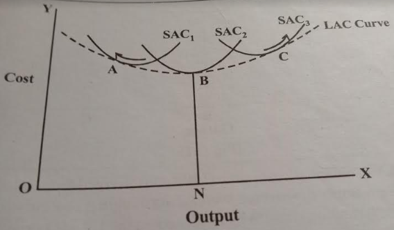
As shown in above Figure, the LAC curve is tangential to SAC1, SAC2, and SAC3 at points A, B, and C respectively. The optimum size plant is shown by SAC2 as at the tangency point B, the cost BN is minimum and the output is = ON. Any other plant has higher AC.
Now, we will discuss about the features of LAC Curve.
Features of LAC Curve:
- The LAC curve like the SAC curve is U shaped but it is flatter than the latter. It is so as the economies which are not possible in the short run become possible in the long run and the diseconomies which cannot be avoided in short period can be avoided in the long run
- When LAC curve is falling it touches the declining part of SAC1 curve to the left of the minimum point and when it is rising it touches the rising part to the right of the minimum point on SAC3.
- No SAC curve can cut LAC curve and lie below it as LAC curve shows minimum cost for any level of output.
- The LAC curve is known as an 'envelope curve' as it envelopes a family of SAC curves.
- The minimum point of SAC2 curve where LAC curve touches it, also becomes the minimum point of LAC curve.
- LAC curve is also called the planning cure as it helps the firm in planning the optimum size of the plant and output.
- The U shape of LAC curve is due to the operation of Laws of Returns.
LAC - Long Average Cost
SAC - Short Average Cost
AC - Average Cost.
CONTINUE READING
Nature of Long run average cost curve
Short run average cost curve
Firm
Factories
Average Cost
Laws of Returns.
Theory of Costs - Nature of Long Run Average Cost Curve (LAC)
Kinnari
Tech writer at NewsandStory